import numpy as np
from matplotlib import pylab as plt
from astropy.io import ascii, fits
from astropy.table import TableWorking with the COSMOS-Web catalog: Example of a few user cases
In this notebook we will present how to use the catalog. We present a few basic user cases such as loading the catalog, selecting a clean/robust sample, plotting the photometry and LePHARE & CIGALE SEDs, and match by coordinates to find a source of interest
Load in the catalog
The catalog is available as COSMOSWeb_mastercatalog_v1.fits on the Download page.
with fits.open('COSMOSWeb_mastercatalog_v1.fits') as hdu:
    hdu.info()
    hdr = hdu[1].header
    cat_photom = Table(hdu[1].data)
    cat_lephare = Table(hdu[2].data)
    cat_cigale = Table(hdu[4].data)
    cat_bd = Table(hdu[6].data)
Filename: /n23data2/cosmosweb/catalogs/Release_v1/COSMOSWeb_mastercatalog_v1.fits
No. Name Ver Type Cards Dimensions Format
0 PRIMARY 1 PrimaryHDU 4 ()
1 PHOTOMETRY HOTCOLD AND SE++ 1 BinTableHDU 603 784016R x 287C [K, K, 3A, K, D, D, D, D, D, D, D, D, D, 4A, D, D, D, D, D, 5D, 5D, 5D, D, D, D, D, D, 5D, 5D, 5D, D, D, D, D, D, 5D, 5D, 5D, D, D, D, D, D, 5D, 5D, 5D, D, D, D, D, D, 5D, 5D, 5D, D, D, D, D, D, 5D, 5D, 5D, D, D, D, D, D, D, D, D, D, D, D, D, D, D, D, D, D, D, D, D, L, L, D, D, D, D, D, D, D, D, D, D, D, D, D, D, D, K, D, D, D, D, D, D, D, D, D, D, D, D, D, D, D, D, D, D, D, D, D, D, D, D, D, D, D, D, D, D, D, D, D, D, D, D, D, D, D, D, D, D, D, D, D, D, D, D, D, D, D, D, D, D, D, D, D, D, D, D, D, D, D, D, D, D, D, D, D, D, D, D, D, D, D, D, D, D, D, D, D, D, D, D, D, D, D, D, D, D, D, D, D, D, D, D, D, D, D, D, D, D, D, D, D, D, D, D, D, D, D, D, D, D, D, D, D, D, D, D, D, D, D, D, D, D, D, D, D, D, D, D, D, D, D, D, D, D, D, D, D, D, D, D, D, D, D, D, I, D, D, D, D, D, D, D, D, D, D, D, D, D, D, D, D, D, D, D, D, D, D, D, D, D, D, D, D, D, D, D, D, D, D, D, D, D, K]
2 LEPHARE 1 BinTableHDU 97 784016R x 43C [D, K, D, D, D, D, D, K, D, D, D, D, D, K, D, K, D, D, D, D, D, D, D, D, D, D, D, D, D, D, D, D, D, D, D, D, D, D, D, D, D, D, D]
3 SE++APER 1 BinTableHDU 454 784016R x 148C [5E, 5E, 5E, 5E, 5E, 5E, 5E, 5E, 5E, 5E, 5E, 5E, 5E, 5E, 5E, 5E, 5E, 5E, 5E, 5E, 5E, 5E, 5E, 5E, 5E, 5E, 5E, 5E, 5E, 5E, 5E, 5E, 5E, 5E, 5E, 5E, 5E, 5E, 5E, 5E, 5E, 5E, 5E, 5E, 5E, 5E, 5E, 5E, 5E, 5E, 5E, 5E, 5E, 5E, 5E, 5E, 5E, 5E, 5E, 5E, 5E, 5E, 5E, 5E, 5E, 5E, 5E, 5E, 5E, 5E, 5E, 5E, 5E, 5E, 5E, 5E, 5E, 5E, 5E, 5E, 5E, 5E, 5E, 5E, 5E, 5E, 5E, 5E, 5E, 5E, 5E, 5E, 5E, 5E, 5E, 5E, 5E, 5E, 5E, 5E, 5E, 5E, 5E, 5E, 5E, 5E, 5E, 5E, 5E, 5E, 5E, 5E, 5E, 5E, 5E, 5E, 5E, 5E, 5E, 5E, 5E, 5E, 5E, 5E, 5E, 5E, 5E, 5E, 5E, 5E, 5E, 5E, 5E, 5E, 5E, 5E, 5E, 5E, 5E, 5E, 5E, 5E, 5E, 5E, 5E, 5E, 5E, 5E]
4 CIGALE 1 BinTableHDU 118 784016R x 54C [D, D, D, D, D, D, D, D, D, D, D, D, D, D, D, D, D, D, D, D, D, D, D, D, D, D, D, D, D, D, D, D, D, D, D, D, D, D, D, D, D, D, D, D, D, D, D, D, D, D, D, D, D, D]
5 ML-MORPHO 1 BinTableHDU 314 784016R x 150C [D, D, D, D, D, D, D, D, D, D, D, D, D, D, D, D, D, D, D, D, D, D, D, D, D, D, D, D, D, D, D, D, D, D, D, D, D, D, D, D, D, D, D, D, D, D, D, D, D, D, D, D, D, D, D, D, D, D, D, D, D, D, D, D, D, D, D, D, D, D, D, D, D, D, D, D, D, D, D, D, D, D, D, D, D, D, D, D, D, D, D, D, D, D, D, D, D, D, D, D, D, D, D, D, D, D, D, D, D, D, D, D, D, D, D, D, D, D, D, D, D, D, D, D, D, D, D, D, D, D, D, D, D, D, D, D, D, D, D, D, D, D, D, D, K, D, K, D, K, D]
6 B+D 1 BinTableHDU 932 784016R x 461C [D, D, D, D, D, D, D, D, D, D, D, D, D, D, D, D, D, D, D, D, D, D, D, D, D, D, D, D, D, D, D, D, D, D, D, D, D, D, D, D, D, D, D, D, D, D, D, D, D, D, D, D, D, D, D, D, D, D, D, D, D, D, D, D, D, D, D, D, D, D, D, D, D, D, D, D, D, D, D, D, D, D, D, D, D, D, D, D, D, D, D, D, D, D, D, D, D, D, D, D, D, D, D, D, D, D, D, D, D, D, D, D, D, D, D, D, D, D, D, D, D, D, D, D, D, D, D, D, D, D, D, D, D, D, D, D, D, D, D, D, D, D, D, D, D, D, D, D, D, D, D, D, D, D, D, D, D, D, D, D, D, D, D, D, D, D, D, D, D, D, D, D, D, D, D, D, D, D, D, D, D, D, D, D, D, D, D, D, D, D, D, D, D, D, D, D, D, D, D, D, D, D, D, D, D, D, D, D, D, D, D, D, D, D, D, D, D, D, D, D, D, D, D, D, D, D, D, D, D, D, D, D, D, D, D, D, D, D, D, D, D, D, D, D, D, D, D, D, D, D, D, D, D, D, D, D, D, D, D, D, D, D, D, D, D, D, D, D, D, D, D, D, D, D, D, D, D, D, D, D, D, D, D, D, D, D, D, D, D, D, D, D, D, D, D, D, D, D, D, D, D, D, D, D, D, D, D, D, D, D, D, D, D, D, D, D, D, D, D, D, D, D, D, D, D, D, D, D, D, D, D, D, D, D, D, D, D, D, D, D, D, D, D, D, D, D, D, D, D, D, D, D, D, D, D, D, D, D, D, D, D, D, D, D, D, D, D, D, D, D, D, D, D, D, D, D, D, D, D, D, D, D, D, D, D, D, D, D, D, D, D, D, D, D, D, D, D, D, D, D, D, D, D, D, D, D, D, D, D, D, D, D, D, D, D, D, D, D, D, D, D, D, D, D, D, D, D, D, D, D, D, D, D, D, D, D, D, D, D, D, D, D, D, D, D, D, D, D, D, D, D, D, D, D, D, D, D, D, D, D, D] Open the LePHARE PDF(z)
These are stored in a pickle file, available as COSMOSWeb_LePHARE_PDFz_v1.pkl on the Download page. It takes a bit of time to load, as its a large file.
import pickle
file = open('COSMOSWeb_LePHARE_PDFz_v1.pkl', 'rb')
# dump information to that file
lephare_pdfz = pickle.load(file)
# close the file
file.close()
Selecting a robust and clean sample of galaxies
The simplest way to select a robust sample of galaxies with reliable photometry and photo-z without sacrificing completeness is the following
condition_clean = np.logical_and.reduce((
    cat_lephare['type']==0, # Select only galaxies
    cat_photom['warn_flag']==0, # No warning flag
    np.abs(cat_photom['mag_model_f444w'])<30, # Remove very faint objects
    cat_photom['flag_star_hsc']==0, # Remove objects in HSC star mask area
))
type is the LePHARE classification 0: galaxy, 1: star, 2: qso. Here we select only galaxies.
Note that because of warn_flag == 0 this excludes sources near bright stars whose photometry in the ground-based data is contaminated by the stars, which yields less reliable photo-z. In the following we plot the spatial distribution of all sources in the catalog, of the clean sample, and of sources with MIRI photometry.
In addition, we also select sources outside of bright stars and which are masked by the HSC star masks. The ground based photometry of these sources can be affected by the bright stars. This is set with flag_star_hsc; 0: good object, 1: masked out
condition_clean_miri = np.logical_and(condition_clean, cat_photom['flux_model_f770w']>0)

fig, ax = plt.subplots(1,1, figsize=(7.5, 6))

ax.hexbin(cat_photom['ra'], cat_photom['dec'], gridsize=160, cmap='gray', mincnt=1)

hb = ax.hexbin(cat_photom[condition_clean]['ra'], cat_photom[condition_clean]['dec'], gridsize=160, cmap='inferno', mincnt=1)
ax.plot(cat_photom[condition_clean_miri]['ra'], cat_photom[condition_clean_miri]['dec'], 'o', ms=1.0, markeredgecolor='None', alpha=1, color='goldenrod')

cb = fig.colorbar(hb, ax=ax)
cb.set_label('N')
ax.set_xlabel('R.A.')
ax.set_ylabel('Dec')
ax.set_xlim(150.65, 149.6)
ax.minorticks_on()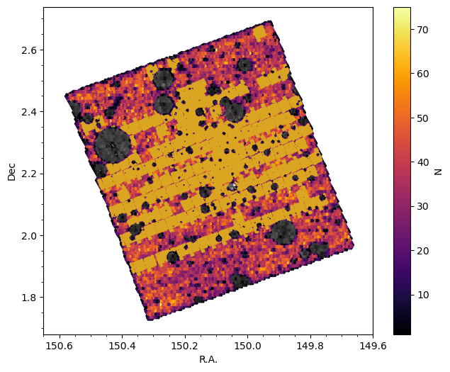
Plot the photometry and SED (from both LePHARE and CIGALE) of a galaxy
The LePHARE SEDs are stored in a directory LePHARE_SEDs_v1/ available as a compressed tar file on the Download page.
The CIGALE SEDs are stored in a directory CIGALE_SEDs_v1/ available as a compressed tar file on the Download page. They are separated into P1, containing galaxies at \(z<5\) and P2, containing galaxies at \(z>5\).
# First, define necessary functions
## Define the filter wavenelghts
filters_lambda_eff_bb = {
'cfht-u' : [0.3690, 0.0456],
'hsc-g' : [0.4851, 0.1194],
'hsc-r' : [0.6241, 0.1539],
'hsc-i' : [0.7716, 0.1476],
'hsc-z' : [0.8915, 0.0768],
'hsc-y' : [0.9801, 0.0797],
'uvista-y' : [1.0222, 0.0919],
'uvista-j' : [1.2555, 0.1712],
'uvista-h' : [1.6497, 0.2893],
'uvista-ks' : [2.1577, 0.2926],
'hst-f814w' : [0.8068, 0.1610],
'f115w' : [1.1622, 0.2646],
'f150w' : [1.5106, 0.3348],
'f277w' : [2.8001, 0.6999],
'f444w' : [4.4366, 1.1109],
'f770w' : [7.7108, 2.0735]}
filters_lambda_eff_nb = {
'sc-ib427' : [0.4264, 0.0207],
'sc-ia484' : [0.4851, 0.0228],
'sc-ib505' : [0.5064, 0.0231],
'sc-ia527' : [0.5262, 0.0242],
'sc-ib574' : [0.5766, 0.0272],
'sc-ia624' : [0.6234, 0.0301],
'sc-ia679' : [0.6783, 0.0336],
'sc-ib709' : [0.7075, 0.0316],
'sc-ia738' : [0.7363, 0.0323],
'sc-ia767' : [0.7687, 0.0364],
'sc-ib827' : [0.8246, 0.0344],
'sc-nb711' : [0.7120, 0.0073],
'sc-nb816' : [0.8150, 0.0120],
'hsc-nb0816' : [0.8168, 0.0110],
'hsc-nb0921' : [0.9205, 0.0133],
'hsc-nb1010' : [1.0100, 0.0094]
}
## Define a function that loads LePHARE SED
def load_lephare_sed(source_id, path="."):
''' Reads the LePHARE SED for a source given its id. Takes only the best-fit SED.
'''
from astropy import units as u
def check_strictly_increasing(arr):
# Check if each element is smaller than the next one
is_increasing = all(x < y for x, y in zip(arr, arr[1:]))
# Find the indices where the array is not strictly increasing
non_increasing_indices = [i for i in range(len(arr) - 1) if arr[i] >= arr[i + 1]]
return is_increasing, non_increasing_indices
# Path to the spectral file
spec_filename = f'{path}/LePHARE_SEDs_v1/Id{source_id}.0.spec'
try:
specfile = np.genfromtxt(spec_filename, skip_header=1551)
## make sure to select only the best-fit galaxy spectrum
is_increasing, non_increasing_indices = check_strictly_increasing(specfile[:,0])
if is_increasing == False:
specfile = specfile[:non_increasing_indices[0], :non_increasing_indices[0]]
# Convert lists to numpy arrays
lambda_um = specfile[:,0]/10000 #converting to microns
mag_ab = specfile[:,1]
# Convert magnitude (AB) to flux density (F_nu) in microJanskys
sed_fnu = (mag_ab * u.ABmag).to(u.uJy).value
return lambda_um, sed_fnu
except Exception as e:
print(f"Error processing source {source_id}: {e}")
return np.linspace(0.1,10, 1000), np.zeros((1000))
# Define a function that loads the CIGALE SED
def load_cigale_sed(source_id, path="."):
'''The CIGALE SEDs are saved in the folder P1 for sources with z<5 and P2 for sources with z>5.
'''
try:
with fits.open(f'{path}/CIGALE_SEDs_v1/P1/{source_id}.0_best_model.fits') as hdu:
cigale_model = hdu[1].data
except:
with fits.open(f'{path}/CIGALE_SEDs_v1/P2/{source_id}.0_best_model.fits') as hdu:
cigale_model = hdu[1].data
return cigale_model
# Define a function to get the PDF(z) from LePHARE for a given source id
def load_lephare_pdfz(source_id, pdz=lephare_pdfz):
'''Function to get the PDF(z) from LePHARE for a given source id.
The PDF(z) are stored in a pickle file which is a dictionary, where the index correponds to the source id
The first array is the redshift array scond array is the Bayesian PDFz, the third one is the likelihood
'''
return pdz[source_id]
def plot_source_photometry_sed(source_id):
''' Takes an id of an individual source and plots the flux for each band and the best-fit SED from both LePHARE and CIGALE
'''
# take the source from the catalog
source_cond = np.where(cat_photom['id']==source_id)
photometry = []
photometry_err = []
band_wave = []
band_wave_width = []
plt.figure(figsize=(7,5), dpi=150)
# loop over each band to load the broad band photometry
for band in filters_lambda_eff_bb:
photometry.append(cat_photom[source_cond][f'flux_model_{band}'][0])
photometry_err.append(cat_photom[source_cond][f'flux_err-cal_model_{band}'][0])
band_wave.append(filters_lambda_eff_bb[band][0])
band_wave_width.append(filters_lambda_eff_bb[band][1])
photometry = np.asarray(photometry)
photometry_err = np.asarray(photometry_err)
band_wave = np.asarray(band_wave)
band_wave_width = np.asarray(band_wave_width)
mask = (photometry/photometry_err>1)
# plot broad band photometry
plt.errorbar(band_wave[mask], photometry[mask], xerr=band_wave_width[mask], yerr=photometry_err[mask], fmt='o', ms=5, color='navy', label='Broad bands')
plt.errorbar(band_wave[~mask], photometry[~mask], yerr=photometry_err[~mask], fmt='o', ms=5, color='navy', label='S/N<1', alpha=0.2)
photometry = []
photometry_err = []
band_wave = []
band_wave_width = []
# loop over each band to load the medium/narrow band photometry
for band in filters_lambda_eff_nb:
photometry.append(cat_photom[source_cond][f'flux_model_{band}'][0])
photometry_err.append(cat_photom[source_cond][f'flux_err-cal_model_{band}'][0])
band_wave.append(filters_lambda_eff_nb[band][0])
band_wave_width.append(filters_lambda_eff_nb[band][1])
photometry = np.asarray(photometry)
photometry_err = np.asarray(photometry_err)
band_wave = np.asarray(band_wave)
band_wave_width = np.asarray(band_wave_width)
mask = (photometry/photometry_err>1)
# plot narrow/medium band photometry
plt.errorbar(band_wave[mask], photometry[mask], xerr=band_wave_width[mask], yerr=photometry_err[mask], fmt='o', alpha=0.6, ms=3, lw=1, color='navy', label='Narrow/medium bands')
plt.errorbar(band_wave[~mask], photometry[~mask], yerr=photometry_err[~mask], fmt='o', ms=3, lw=1, color='navy', alpha=0.2)
### write properties
idd = cat_photom[source_cond]['id'][0]
z = cat_lephare[source_cond]['zfinal'][0]
mass = cat_lephare[source_cond]['mass_med'][0]
ssfr = cat_lephare[source_cond]['ssfr_med'][0]
nuvr = cat_lephare[source_cond]['mabs_nuv'][0]-cat_lephare[source_cond]['mabs_r'][0]
rj = cat_lephare[source_cond]['mabs_r'][0]-cat_lephare[source_cond]['mabs_j'][0]
plt.text(x=0.33,y=0.8,s=
fr'id = {idd}'
'\n'
fr'$z$ = {z:.2f}'
'\n'
r'log$M_{\star}/{\rm M_{\odot}} = $'+f'{mass:.2f}'
'\n'
r'log sSFR$/$yr$^{-1} = $'+f'{ssfr:.2f}'
'\n'
fr'$NUV-r$ = {nuvr:.2f}'
'\n'
fr'$r-J$ = {rj:.2f}'
,fontsize=10) #,bbox=dict(facecolor='white'))
# load and plot LePHARE SED
lambda_lephare, sed_lephare = load_lephare_sed(source_id)
plt.plot(lambda_lephare, sed_lephare, color='tomato', label='LePHARE SED', lw=2, zorder=-10)
# load and plot CIGALE SED
try:
cigale_model = load_cigale_sed(source_id)
plt.plot(cigale_model['wavelength']/1000, (cigale_model['Fnu']*1.0e3),
lw=2, alpha=0.7, color='goldenrod', label='CIGALE SED', zorder=-11)
except:
print('Can not find CIGALE output for this source')
plt.xlim(0.3, 10)
plt.ylim(0.001, 10)
plt.xscale('log')
plt.yscale('log')
plt.xlabel(r'Wavelength [$\mu$m]')
plt.ylabel(r'Flux [$\mu$Jy]')
plt.legend(loc=4)
plt.minorticks_on()
plt.show()
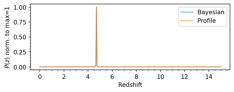
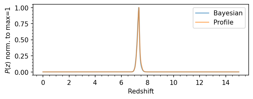
# Plot the PDF(z)
pdfz = load_lephare_pdfz(source_id)
plt.figure(figsize=(6,2), dpi=150)
plt.plot(pdfz[0,:], pdfz[1,:]/np.max(pdfz[1,:]), label='Bayesian', alpha=0.6)
plt.plot(pdfz[0,:], pdfz[2,:]/np.max(pdfz[2,:]), label='Profile', alpha=0.6)
plt.xlabel(r'Redshift')
plt.ylabel(r'$P(z)$ norm. to max=1')
plt.legend()
plt.minorticks_on()
plt.show()
return
plot_source_photometry_sed(564339)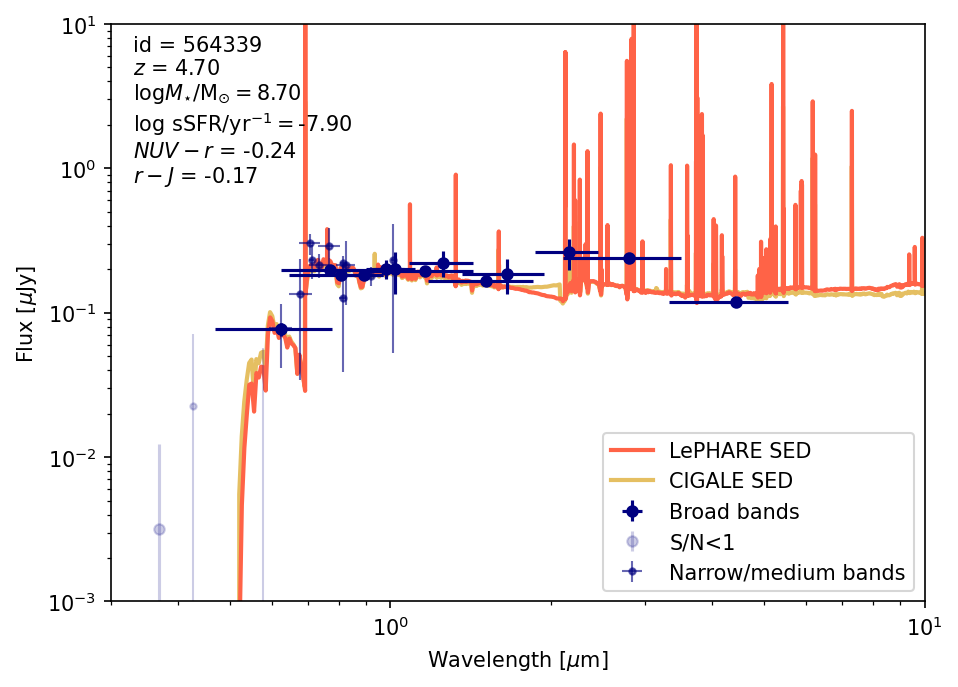
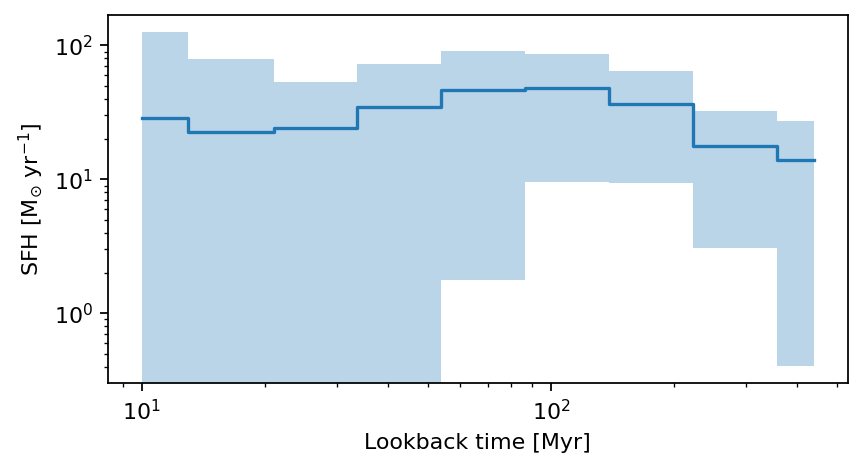
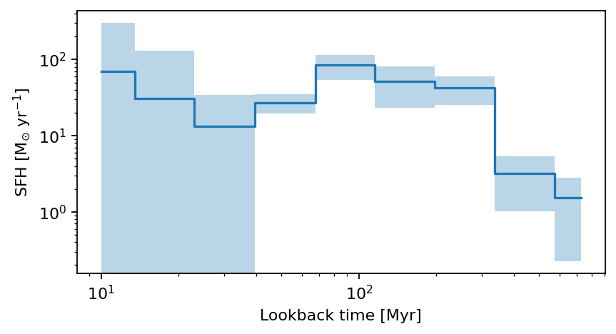
Plot the non-parametric SFH from CIGALE
def plot_cigale_sfh(source_id):
    ''' Plots the non-parametric SFH from CIGALE for a given source id
    '''

    fig, ax = plt.subplots(dpi=159, figsize=(6, 3))  # Create figure and axes


    source_cond = np.where(cat_photom['id']==source_id)

    # define the SFH column names
    yy = ('sfh_sfr_bin1', 'sfh_sfr_bin2', 'sfh_sfr_bin3', 'sfh_sfr_bin4', 'sfh_sfr_bin5', 'sfh_sfr_bin6', 'sfh_sfr_bin7', 'sfh_sfr_bin8', 'sfh_sfr_bin9')
    yy_err = ('sfh_sfr_bin1_err', 'sfh_sfr_bin2_err', 'sfh_sfr_bin3_err', 'sfh_sfr_bin4_err', 'sfh_sfr_bin5_err', 'sfh_sfr_bin6_err', 'sfh_sfr_bin7_err', 'sfh_sfr_bin8_err',   'sfh_sfr_bin9_err')
    xx = ('sfh_time_bin1', 'sfh_time_bin2', 'sfh_time_bin3', 'sfh_time_bin4', 'sfh_time_bin5', 'sfh_time_bin6', 'sfh_time_bin7', 'sfh_time_bin8', 'sfh_time_bin9'   )

    x = np.array([cat_cigale[source_cond][xx_][0] for xx_ in xx])
    y = np.array([cat_cigale[source_cond][xx_][0] * cat_cigale[source_cond]['sfh_integrated'][0] for xx_ in yy])
    y_err = np.array([cat_cigale[source_cond][xx_][0] * cat_cigale[source_cond]['sfh_integrated'][0] for xx_ in yy_err])

    ax.step(x, y, where='mid')
    ax.fill_between(x, y - y_err, y + y_err, alpha=0.3, step='mid')

    ax.set_xscale('log')
    ax.set_yscale('log')
    # ax.set_ylim(1.e-14, 1.e-8)
    ax.minorticks_on()
    ax.set_xlabel('Lookback time [Myr]')
    ax.set_ylabel(r'SFH [M$_{\odot}$ yr$^{-1}$]')

    plt.show()

    return

plot_cigale_sfh(564339)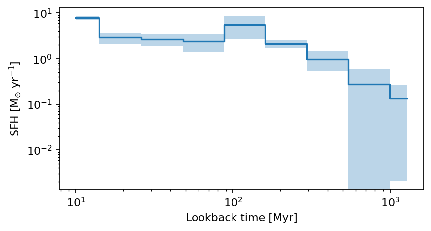
Use R.A. and Dec of a source published in the literature and plot its photometry and SED
For this example we will plot SEDs for one of the high-\(z\) bright/massive candidates from Casey et al. (2024) and the dusty star-forming galaxy REBELS-25 (Rowland et al. 2024). We will use the coordinates to find a match in the catalog and look at its photometry, SED, SFH and properties.
- Source 1: Casey et al. 2024, (COS-z10-4) RA,Dec: [150.158166666 1.825675] \(z= 10.58 \pm 0.13\)
- Source 2: REBELS-2) RA,Dec: [150.24371, 1.83222] \(z_{\rm spec}=7.09\)
from astropy.coordinates import SkyCoord
from astropy import units as u


# Define source coordinates
ra_source1 = 150.158166666
dec_source1 = 1.825675
# Match coordinates with the catalog
reference_catalog = SkyCoord(ra=cat_photom['ra']*u.degree, dec=cat_photom['dec']*u.degree)
source =  SkyCoord(ra=ra_source1*u.degree, dec=dec_source1*u.degree)
idx, _, _ = source.match_to_catalog_sky(reference_catalog)
# plot
source_id_source1 = cat_photom['id'][idx]
plot_source_photometry_sed(source_id_source1)
plot_cigale_sfh(source_id_source1)

## REBELS-25

# Define source coordinates
ra_source2 = 150.24371
dec_source2 = 1.83222
# Match coordinates with the catalog
reference_catalog = SkyCoord(ra=cat_photom['ra']*u.degree, dec=cat_photom['dec']*u.degree)
source =  SkyCoord(ra=ra_source2*u.degree, dec=dec_source2*u.degree)
idx, _, _ = source.match_to_catalog_sky(reference_catalog)

# plot
source_id_source2 = cat_photom['id'][idx]
plot_source_photometry_sed(source_id_source2)
plot_cigale_sfh(source_id_source2)
Display detailed inspection plots
As part of the catalog release, we also provide detailed inspection plots for each source. These plots show image stamps in different bands, the detection image and segmentation map, and plot the photometry, best-fit SED, and physical parameters. These are included in the Interactive Map Viewer here
For a given source ID sid, inspection plots can be found on the following link:
https://cosmos2025.iap.fr/fitsmap/data/inspec_plots/cosmos_web_sed_{sid}.pdf
In the following we demostrate how to display them easily. We will use the sources from the examples above
from IPython.display import IFrame
pdf_url_sourceid = lambda sid: f"https://cosmos2025.iap.fr/fitsmap/data/inspec_plots/cosmos_web_sed_{sid}.pdf"

IFrame(pdf_url_sourceid(564339), width=1000, height=650)IFrame(pdf_url_sourceid(358243), width=1000, height=650)Plot some statistical distributions
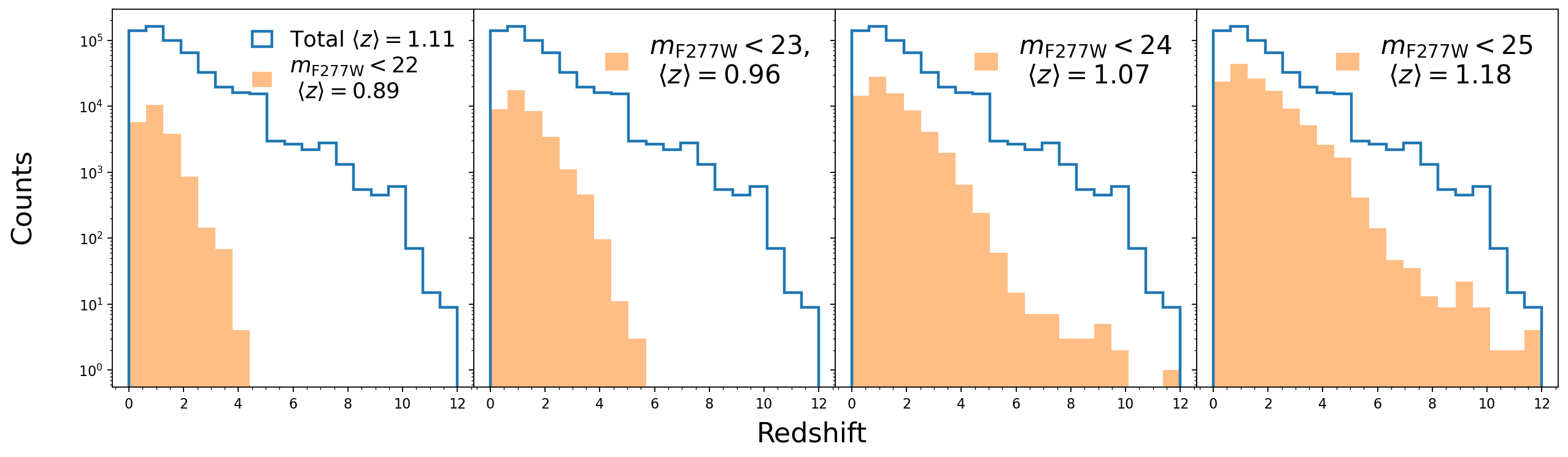
- Redshift distribution for the full sample and magnitude-selected samples
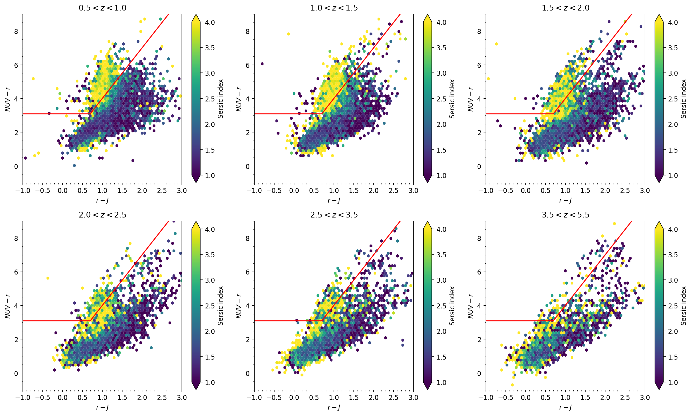
- NUV-r-J diagram color coded by the sersic index, in a few redshift bins
fig, axs = plt.subplots(1, 4, dpi=160, figsize=(19, 5), sharex=True, sharey=True)
plt.subplots_adjust(wspace=0, hspace=0)
axs = axs.ravel()

cond_clean = (cat_lephare['type']==0) & (cat_photom['warn_flag']==0) & (np.abs(cat_photom['mag_model_f444w'])<30) & (cat_photom['flag_star_hsc']==0)
cond_mag0 = cond_clean & (cat_photom['mag_model_f277w'] < 22)
cond_mag1 = cond_clean & (cat_photom['mag_model_f277w'] < 23)
cond_mag2 = cond_clean & (cat_photom['mag_model_f277w'] < 24)
cond_mag3 = cond_clean & (cat_photom['mag_model_f277w'] < 25)


zmed_tot = np.around(np.median(cat_lephare['zfinal'][cond_clean]),2)
zmed_mag = np.around(np.median(cat_lephare['zfinal'][cond_mag0]),2)
axs[0].hist(cat_lephare['zfinal'][cond_clean], bins=np.linspace(0,12,20), histtype='step', label=r'Total'+f' $\\langle z \\rangle=${zmed_tot}', lw=2, density=False)
axs[0].hist(cat_lephare['zfinal'][cond_mag0], bins=np.linspace(0,12,20), label=r'$m_{\rm F277W} < 22$'+f' \n $\\langle z \\rangle=${zmed_mag}', density=False, alpha=0.5, histtype='stepfilled')

zmed_mag = np.around(np.median(cat_lephare['zfinal'][cond_mag1]),2)
axs[1].hist(cat_lephare['zfinal'][cond_clean], bins=np.linspace(0,12,20), histtype='step', lw=2, density=False)
axs[1].hist(cat_lephare['zfinal'][cond_mag1], bins=np.linspace(0,12,20), label=r'$m_{\rm F277W} < 23$, '+f'\n $\\langle z \\rangle=${zmed_mag}', density=False, alpha=0.5, histtype='stepfilled')

zmed_mag = np.around(np.median(cat_lephare['zfinal'][cond_mag2]),2)
axs[2].hist(cat_lephare['zfinal'][cond_clean], bins=np.linspace(0,12,20), histtype='step', lw=2, density=False)
axs[2].hist(cat_lephare['zfinal'][cond_mag2], bins=np.linspace(0,12,20), label=r'$m_{\rm F277W} < 24$'+f' \n $\\langle z \\rangle=${zmed_mag}', density=False, alpha=0.5, histtype='stepfilled')

zmed_mag = np.around(np.median(cat_lephare['zfinal'][cond_mag3]),2)
axs[3].hist(cat_lephare['zfinal'][cond_clean], bins=np.linspace(0,12,20), histtype='step', lw=2, density=False)
axs[3].hist(cat_lephare['zfinal'][cond_mag3], bins=np.linspace(0,12,20), label=r'$m_{\rm F277W} < 25$'+f' \n $\\langle z \\rangle=${zmed_mag}', density=False, alpha=0.5, histtype='stepfilled')

for i in [0,1,2,3]:
    axs[i].set_yscale('log')
    axs[i].minorticks_on()
    # axs[i].set_ylim(1.e-5, 4)
    if i == 0:
        axs[i].legend(fontsize=16, handlelength=0.9, labelspacing=0.2, loc=1, frameon=False)
    else:
        axs[i].legend(fontsize=19, handlelength=0.9, labelspacing=0.2, loc=1, frameon=False)
    axs[i].set_xticks([0, 2, 4, 6, 8, 10, 12], [0, 2, 4, 6, 8, 10, 12])
fig.text(0.5, -0.001, f'Redshift', ha='center', fontsize=20)
fig.text(0.07, 0.5, 'Counts', va='center', rotation='vertical', fontsize=20)
# plt.tight_layout()
plt.show()
fig, axs = plt.subplots(2, 3, dpi=160, figsize=(15, 9))
axs = axs.ravel()

cond_clean = (cat_lephare['type']==0) & (cat_photom['warn_flag']==0) & (cat_photom['flux_model_f444w']/cat_photom['flux_err-cal_model_f444w']>5) & (cat_photom['flag_star_hsc']==0)
cond_z1 = cond_clean & (cat_lephare['zfinal'] >= 0.5) & (cat_lephare['zfinal'] < 1.0) & (cat_lephare['mass_med'] > 9.5)
cond_z2 = cond_clean & (cat_lephare['zfinal'] >= 1.0) & (cat_lephare['zfinal'] < 1.5) & (cat_lephare['mass_med'] > 9.5)
cond_z3 = cond_clean & (cat_lephare['zfinal'] >= 1.5) & (cat_lephare['zfinal'] < 2.0) & (cat_lephare['mass_med'] > 9.5)
cond_z4 = cond_clean & (cat_lephare['zfinal'] >= 2.0) & (cat_lephare['zfinal'] < 2.5) & (cat_lephare['mass_med'] > 9.5)
cond_z5 = cond_clean & (cat_lephare['zfinal'] >= 2.5) & (cat_lephare['zfinal'] < 3.5) & (cat_lephare['mass_med'] > 9.5)
cond_z6 = cond_clean & (cat_lephare['zfinal'] >= 3.5) & (cat_lephare['zfinal'] < 5.5) & (cat_lephare['mass_med'] > 9.5)


axs[0].set_title(r'$0.5<z<1.0$')
hb = axs[0].hexbin(cat_lephare['mabs_r'][cond_z1]-cat_lephare['mabs_j'][cond_z1],
              cat_lephare['mabs_nuv'][cond_z1]-cat_lephare['mabs_r'][cond_z1],
                mincnt=1, extent=(-1,3, -1, 9), linewidths=0, C=cat_photom[cond_z1]['sersic'], vmin=1, vmax=4, gridsize=60)
cb = fig.colorbar(hb, ax=axs[0], label='Sersic index', extend="both")


axs[1].set_title(r'$1.0<z<1.5$')
hb = axs[1].hexbin(cat_lephare['mabs_r'][cond_z2]-cat_lephare['mabs_j'][cond_z2],
              cat_lephare['mabs_nuv'][cond_z2]-cat_lephare['mabs_r'][cond_z2],
              mincnt=1, extent=(-1,3, -1, 9), linewidths=0, C=cat_photom[cond_z2]['sersic'], vmin=1, vmax=4, gridsize=60)
cb = fig.colorbar(hb, ax=axs[1], label='Sersic index', extend="both")


axs[2].set_title(r'$1.5<z<2.0$')
hb = axs[2].hexbin(cat_lephare['mabs_r'][cond_z3]-cat_lephare['mabs_j'][cond_z3],
              cat_lephare['mabs_nuv'][cond_z3]-cat_lephare['mabs_r'][cond_z3],
              mincnt=1, extent=(-1,3, -1, 9), linewidths=0, C=cat_photom[cond_z3]['sersic'], vmin=1, vmax=4, gridsize=60)
cb = fig.colorbar(hb, ax=axs[2], label='Sersic index', extend="both")


axs[3].set_title(r'$2.0<z<2.5$')
hb = axs[3].hexbin(cat_lephare['mabs_r'][cond_z4]-cat_lephare['mabs_j'][cond_z4],
              cat_lephare['mabs_nuv'][cond_z4]-cat_lephare['mabs_r'][cond_z4],
              mincnt=1, extent=(-1,3, -1, 9), linewidths=0, C=cat_photom[cond_z4]['sersic'], vmin=1, vmax=4, gridsize=60)
cb = fig.colorbar(hb, ax=axs[3], label='Sersic index', extend="both")


axs[4].set_title(r'$2.5<z<3.5$')
hb = axs[4].hexbin(cat_lephare['mabs_r'][cond_z5]-cat_lephare['mabs_j'][cond_z5],
              cat_lephare['mabs_nuv'][cond_z5]-cat_lephare['mabs_r'][cond_z5],
              mincnt=1, extent=(-1,3, -1, 9), linewidths=0, C=cat_photom[cond_z5]['sersic'], vmin=1, vmax=4, gridsize=60)
cb = fig.colorbar(hb, ax=axs[4], label='Sersic index', extend="both")


axs[5].set_title(r'$3.5<z<5.5$')
hb = axs[5].hexbin(cat_lephare['mabs_r'][cond_z6]-cat_lephare['mabs_j'][cond_z6],
              cat_lephare['mabs_nuv'][cond_z6]-cat_lephare['mabs_r'][cond_z6],
              mincnt=1, extent=(-1,3, -1, 9), linewidths=0, C=cat_photom[cond_z6]['sersic'], vmin=1, vmax=4, gridsize=60)
cb = fig.colorbar(hb, ax=axs[5], label='Sersic index', extend="both")


for i in range(6):
    axs[i].plot([-2,0.7],[3.1,3.1], c='red')
    axs[i].plot([0.7,5.7],3*np.array([0.7,5.7])+1, c='red')
    axs[i].set_ylim(-1,9)
    axs[i].set_xlim(-1,3)
    axs[i].set_xlabel(r'$r-J$')
    axs[i].set_ylabel(r'$NUV - r$')
    axs[i].minorticks_on()
plt.tight_layout()
plt.show()